Examples of Data Analysis and Machine Learning

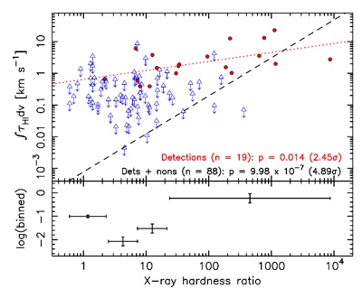
When an object is undetected in observational astronomy it does not necessarily mean that the object is not there, but is emitting radiation too faint to be detected with the instrument. Thus, upper limits to the measurement may feature more often in the data than the detected measurements themselves, such as in the plot below. These data can prove very useful and may be incorporated via survival analysis, which gives a  maximum-likelihood estimate based upon the parent population .

In the example shown, the correlation between the density of star-forming gas (HI) in the host galaxy  and the attenuation of X-ray emission from the central super-massive black hole is barely significant from the detections alone (red circles). However, when the upper limits to the gas density are included (blue triangles), the probability of the distribution arising by chance drops from 1.4% to a one in a million. Published in Moss et al, (2017).

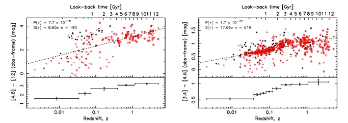
The plots below (published in Curran & Duchesne, 2018) show how a given galaxy ‘colour’ is correlated with redshift (spanning 12 billion years of cosmic history). Both are highly significant, with the left having a ‘p-value’ of p = 7.7 x 10-18 and the right p = 4.7 x 10-70 . This suggests that the relationship on the right may be the more significant, but this is based upon 619 galaxies, compared to 190 on the left. One could select 190 galaxies at random from the 619 to test this, although one trial could lead to a(n) (un)lucky result. I therefore performed a Monte Carlo simulation with 10,000 trials, selecting a random 190 of the 619 each trial and recording the significance of the correlation, which gave a mean ‘Z-value’ of S(τ) = (9.79 +/- 0.92)σ. The bottom end of this range is close to the  S(τ) =  8.60σ for the data on the left, suggesting that the correlations would be similar for the same sized sample.

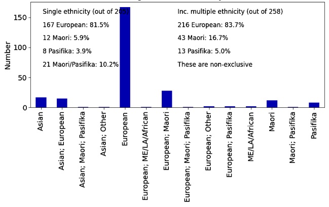
While I have used such tests extensively in the context of extragalactic astrophysics (e.g. Curran et al., 2019), I have also applied these to student evaluation data (Curran 2020) and student populations in tertiary eduction. The plot below shows the distribution of students by ethnicity for the 2021 intake at a particular school for a New Zealand university. Like all universities, they strive to the reach the national fraction of Maori (16.5%) and Pasifika (8.1%) students.

Regression (incorporating limits)

Here I give some examples of the data analysis, statistical techniques and machine learning (often with large, cumbersome, inhomogeneous datasets) I have used in my research and elsewhere. Note that most of the graphics have been written by myself in C.

Monte Carlo Simulations

AB Testing/T-Statistics/Binomial Probabilities

For the students which identify with a single ethnicity, at 10.2%, the Maori/Pasifika (Maori + Pasifika + Maori; Pasifika) is well below the national level of 24.6%, although the binomial probability of 56 Maori + Pasifika students or fewer out of 258 (21.7%) is p = 0.157. This is significant at just 1.01σ and so for this particular school, at least where the students identify with more than one ethnicity, the Maori + Pasifika fraction is consistent with the national level. This method was also used to compare the fractions between schools, each with a very different number of students.

Classification with Machine Learning

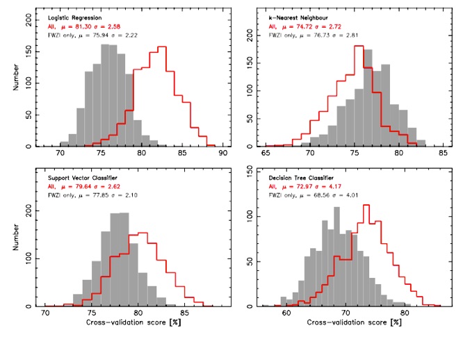
As mentioned under Current Research, the traditional use of an optical spectrum to yield the redshift (and hence distance) of a source can lead to selection biases. Furthermore, such methods will be completely impractical for the millions of new sources expected to be discovered with forthcoming large radio survey (with the Square Kilometre Array and its precursors). I have therefore explored machine learning techniques to classify the nature of a spectrum detected in the radio band - whether the light is absorbed by gas associated with the host galaxy of the radio source itself or arises from a nearer galaxy intervening its line-of-sight. Knowing this is crucial in determining whether the cold gas (which forms all of the stars) arises in a quiescent galaxy, like our own Milky Way, or an active galaxy (quasar), which is powered by a super-massive black hole.

Although the training dataset is very small (with only 56 intervening and 80 associated cases), via random under-sampling of 56 of the associated absorbers prior to each of the 1000 trials, we find that Logistic Regression has a > 80% accuracy (Curran 2021).  While not exceedingly high, this is based upon a very small sample and is still much better than a 50% guess. We expect the accuracy to increase significantly as more and more detections are added to the training sample in the next few years.

Deep Learning (Artificial Neural Networks)

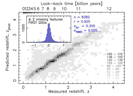
In Curran et al. (2021) I demonstrated the superiority of Deep Learning over other Machine Learning techniques (k-Nearest Neighbour & Decision Tree Regression) in using the  brightness of a quasar in various bands (near-infrared, optical & ultra-violet) to determine its redshift. As mentioned above, current spectroscopic methods are observationally expensive and will be impractical for the vast number of new objects which will be discovered with forthcoming surveys.

Unlike other studies, I have shown that training a large optically-selected dataset (100,000 sources) can provide accurate redshift predictions for radio-selected datasets, thus having the potential to determine the cosmological distances of sources detected in large upcoming surveys in various observing bands.

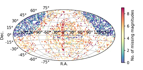
However, the requirement  of nine features (magnitudes) per source can cut the sample sizes by up to 50%, thus limiting the potential of the Deep Learning. Using Machine Learning to impute the missing data, I have shown that up to two missing features can be imputed without significant detriment to the predictions, while  returning > 80% of the sample (Curran, 2022).